Introduction
Businesses generate enormous amounts of customer data every day, but raw data alone rarely answers the questions that matter most:
- Which customers share similar financial behaviors?
- Which groups are more likely to respond to certain products?
- How can organizations personalize services without manually analyzing thousands of records?
- Are there hidden patterns that traditional reporting fails to uncover?
These questions are at the heart of customer segmentation, one of the most valuable applications of data science. Rather than treating every customer the same, organizations can divide their customer base into meaningful groups and make smarter business decisions based on those insights.
Customer segmentation powers many of the experiences we encounter every day. Banks use it to design financial products, retailers personalize promotions, insurance companies assess customer profiles, and marketing teams create campaigns tailored to specific audiences.
In this project, I built an end-to-end customer segmentation pipeline using Python and several machine learning techniques. Starting with the 2019 Survey of Consumer Finances (SCF) dataset published by the Federal Reserve, I explored household financial data, applied K-Means clustering to discover natural customer groups, reduced high-dimensional data using Principal Component Analysis (PCA) for visualization, and finally deployed an interactive Dash web application on Render.
Instead of producing a static notebook, I wanted users to experiment with the model themselves. The dashboard allows visitors to:
- Choose between trimmed variance and raw variance for feature selection.
- Adjust the number of clusters (K) using an interactive slider.
- View real-time clustering metrics such as inertia and silhouette score.
- Explore an interactive PCA visualization of customer segments.
- Compare the financial characteristics of each cluster through dynamically generated charts.
This project demonstrates not only machine learning techniques but also the complete workflow of transforming a data science model into a user-friendly application that anyone can interact with through a web browser.
Project Overview
The primary objective of this project was to identify meaningful groups of U.S. households based on their financial characteristics using unsupervised machine learning. Unlike supervised learning, where models learn from labeled examples, this dataset contained no predefined customer categories. Instead, the goal was to allow the algorithm to discover naturally occurring groups based solely on similarities in financial behavior.
The project followed a structured data science workflow consisting of four major stages:
- Exploratory Data Analysis (EDA) to understand the dataset and identify important variables.
- K-Means clustering using a small set of features before expanding to multiple financial variables.
- Principal Component Analysis (PCA) to visualize high-dimensional clusters in two dimensions.
- Interactive dashboard development using Dash and Plotly, enabling users to experiment with clustering parameters in real time.
Rather than treating each notebook as a separate exercise, together they form a complete machine learning pipeline from raw data exploration to a deployed analytical application.
Dataset
This project uses data from the 2019 Survey of Consumer Finances (SCF), a nationally recognized survey conducted by the Federal Reserve Board to study the financial characteristics of U.S. households.
The dataset contains detailed information on income, debt, assets, net worth, housing, education, retirement savings, and many other financial indicators. For this project, I narrowed the analysis to households that met two important criteria:
- They had been turned down for credit or feared being denied credit within the past five years (TURNFEAR == 1).
- Their net worth was below $2 million, helping focus the analysis on households with more comparable financial profiles while reducing the influence of extreme wealth outliers.
Filtering the data in this way made the clustering process more meaningful by concentrating on a specific population facing similar financial challenges. Among the many available variables, the project focused on several key financial indicators, including:
- INCOME — Total household income
- NETWORTH — Household net worth (assets minus liabilities)
- DEBT — Total household debt
- CCBAL — Credit card balance
- HOUSES — Value of the primary residence
- MRTHEL — Mortgage debt on the primary residence
- NFIN — Total non-financial assets
- RETQLIQ — Retirement account balances
- AGE — Age of household head
- EDUC — Education level
- NHNFIN — Non-home non-financial assets
Together, these variables provide a comprehensive view of a household's financial situation, making them well suited for discovering patterns that may not be immediately visible through traditional statistical analysis.
Why Customer Segmentation Matters
Organizations rarely benefit from treating every customer as though they have identical needs. Two customers might earn similar incomes but differ dramatically in debt levels, home ownership, retirement savings, or financial risk. Marketing the same product to both customers would likely produce very different outcomes.
Customer segmentation solves this problem by grouping customers with similar characteristics. Instead of asking: "What does the average customer look like?" we instead ask: "What different types of customers exist?"
This shift in perspective enables organizations to create strategies tailored to each segment rather than relying on broad assumptions. For example, financial institutions can use segmentation to:
- Identify customers who may qualify for specific loan products.
- Detect groups with high debt but stable income.
- Understand households with strong savings but limited investments.
- Design personalized financial education programs.
- Improve customer retention through targeted recommendations.
Retail companies can segment customers based on purchasing behavior, while healthcare organizations can group patients with similar risk profiles. The underlying principle remains the same: uncover hidden patterns that lead to better decision-making.
Because the dataset used in this project did not include predefined customer categories, unsupervised learning was the ideal approach.
Understanding Unsupervised Learning
Machine learning is often divided into two major categories:
Supervised Learning
In supervised learning, the model learns from labeled examples. Here, the algorithm already knows the correct outcome and learns to predict it for future observations. Common supervised learning tasks include: Spam detection, House price prediction, Disease diagnosis, Fraud detection, and Sentiment analysis.
The previous projects in my portfolio, such as Fraud Detection and NLP Sentiment Analysis, fall into this category because they rely on labeled data to make predictions.
Unsupervised Learning
In contrast, unsupervised learning works without labeled outcomes. The model receives only the input data and attempts to discover patterns on its own. Imagine placing hundreds of customer profiles on a table without any labels. Rather than predicting an answer, the algorithm looks for similarities and groups customers based on shared characteristics.
This makes unsupervised learning particularly useful for tasks such as: Customer segmentation, Recommendation systems, Market basket analysis, Anomaly detection, Topic modeling, and Image compression.
Among the many clustering algorithms available, K-Means remains one of the most widely used because it is intuitive, computationally efficient, and performs well for many practical segmentation problems.
Exploring the Data
Before applying any machine learning algorithm, it's essential to understand the data you're working with. Even the most sophisticated model will struggle if the underlying data contains inconsistencies, outliers, or poorly chosen features.
That's why the first notebook in this project focused entirely on Exploratory Data Analysis (EDA). Rather than jumping straight into clustering, I examined the financial characteristics of the households, identified important variables, and explored relationships that would later influence feature selection.
This stage serves two important purposes:
- It helps uncover patterns that may already exist within the data.
- It provides the insight needed to make informed preprocessing and modeling decisions.
Skipping EDA often leads to models that are difficult to interpret or produce misleading results. By understanding the data first, we can build a more reliable and meaningful segmentation model.
Filtering the Dataset
The original Survey of Consumer Finances contains thousands of observations across hundreds of variables describing different aspects of household finances. For this project, I narrowed the focus to households that satisfied two conditions:
- TURNFEAR == 1, meaning the household had either been denied credit or feared being denied credit in the previous five years.
- NETWORTH < $2,000,000, which excluded extremely wealthy households whose financial profiles could disproportionately influence the clustering process.
These filters were intentional. The first condition targeted households experiencing some level of credit insecurity, making the segmentation more relevant for understanding financial behavior within this specific population.
The second condition reduced the impact of extreme outliers. Financial datasets often contain a small number of observations with exceptionally high incomes or net worth, and these values can dominate statistical measures such as variance and distance calculations. By focusing on households below the $2 million threshold, the resulting clusters better represent typical financial profiles rather than being skewed by a handful of exceptionally wealthy individuals.
Understanding Feature Distributions
Once the dataset had been filtered, I explored the distributions of several key variables, including: Household income, Net worth, Total debt, Credit card balances, Home values, Mortgage balances, Retirement savings, Age, and Education level.
Visualizing these variables revealed an important characteristic of financial data: most financial features are heavily skewed. For example, household income is rarely distributed evenly. Many households earn moderate incomes, while a much smaller number earn significantly more. The same pattern often appears with net worth, debt, and asset values.
This type of skewed distribution is common in real-world financial datasets and presents challenges for machine learning algorithms that rely on distance calculations. Without understanding these distributions, it's easy to assume that every feature contributes equally to clustering when, in reality, variables with extreme values can dominate the results.
Investigating Relationships between Variables
Another important step involved examining how different financial variables relate to one another. Using correlation analysis, I explored relationships such as:
- Income versus net worth
- Debt versus mortgage balances
- Home values versus mortgage debt
- Assets versus retirement savings
Correlation does not imply causation, but it does help identify variables that move together. For instance, households with higher home values often carry larger mortgages, while higher incomes may correlate with larger retirement savings. Understanding these relationships helps determine whether multiple variables provide unique information or simply repeat similar patterns.
Although K-Means does not require independent features, recognizing strong relationships between variables is useful when interpreting the final clusters.
Measuring Feature Variability
One of the most important questions in customer segmentation is: Which features actually help distinguish one household from another?
Variables that show little variation across households contribute relatively little to clustering because they don't provide enough information to separate observations. Conversely, variables with greater variability often capture meaningful differences between customers. To identify these informative variables, I calculated the variance for each financial feature.
Variance measures how spread out the values of a variable are around their average. A simple way to think about it is:
- Low variance means most households have similar values.
- High variance means households differ substantially.
Features with higher variance tend to be more useful because they contain more information that can help separate observations into distinct groups. However, financial data introduces an important complication.
Why Raw Variance Isn't Always Enough
Suppose nearly every household in a dataset has an income between $40,000 and $90,000, but one household earns $20 million. That single observation dramatically increases the calculated variance, making income appear far more variable than it truly is for most households.
This is a classic example of outlier influence. Financial datasets frequently contain extreme values:
- Very wealthy households
- Exceptionally large investment portfolios
- High-value real estate
- Large inheritances
- Unusually high debts
While these observations are valid, they may not represent the majority of the population. If feature selection relies solely on raw variance, the chosen variables can be heavily influenced by these rare cases. To address this challenge, the project also incorporated trimmed variance.
What Is Trimmed Variance?
Trimmed variance is a more robust alternative to standard variance. Instead of using every observation, trimmed variance removes a small percentage of the highest and lowest values before performing the calculation.
In this project, trimming reduces the influence of extreme outliers while preserving the overall structure of the data. The benefits include:
- More representative estimates of variability
- Reduced sensitivity to unusually large financial values
- More stable feature selection
- Better clustering performance for typical households
Rather than asking, "Which variables have the largest values?" trimmed variance asks, "Which variables vary the most for the majority of households?" This distinction becomes especially valuable when working with real-world financial datasets, where outliers are common.
Selecting the Most Informative Features
After comparing both raw and trimmed variance, I ranked the financial variables according to how much they varied across households. Instead of feeding every available variable into the clustering algorithm, I selected the top five high-variance features.
This approach offers several advantages:
- It reduces computational complexity.
- It minimizes noise from less informative variables.
- It focuses the model on the characteristics that best differentiate households.
- It simplifies interpretation of the resulting customer segments.
Feature selection is often overlooked in unsupervised learning, but it's just as important as it is in supervised machine learning. Including too many irrelevant or low-information variables can make clusters less meaningful and harder to interpret.
The selected features then became the foundation for the next stage of the project.
Building an Intuition for K-Means
Before clustering households using multiple financial variables, I wanted to understand how the algorithm behaves in a simpler setting. Instead of immediately working with high-dimensional data, I began by clustering using only two financial features.
Reducing the problem to two dimensions makes it much easier to visualize:
- How clusters are formed.
- Where cluster boundaries emerge.
- How centroids move during training.
- How changing the number of clusters affects the results.
This intermediate step serves as an excellent bridge between exploratory analysis and full-scale customer segmentation. It also provides an intuitive understanding of the mechanics behind K-Means clustering before introducing additional complexity with multiple features and Principal Component Analysis (PCA).
Building Customer Segments with K-Means Clustering
With a solid understanding of the data and the most informative financial features identified, the next step was to uncover natural groupings of households. Since the dataset contained no predefined labels, this called for an unsupervised learning algorithm capable of discovering patterns based solely on similarities within the data.
For this project, I chose K-Means clustering, one of the most widely used clustering algorithms due to its simplicity, efficiency, and interpretability. The implementation was divided into two stages:
- First, clustering with two features to understand the algorithm visually.
- Then, clustering with multiple financial variables to build a more realistic segmentation model.
This progression made it easier to understand how K-Means behaves before scaling up to higher-dimensional data.
What Is K-Means Clustering?
K-Means is an algorithm that groups similar observations into K distinct clusters. Rather than being told what each customer represents, the algorithm discovers groups by measuring how similar households are to one another.
The basic workflow looks like this:
- Choose the desired number of clusters (K).
- Randomly initialize K centroids.
- Assign every household to its nearest centroid.
- Recalculate the centroid of each cluster.
- Repeat the assignment and update steps until the centroids stop moving significantly.
The result is a set of clusters where households within the same group are more similar to each other than they are to households in other groups. For customer segmentation, this means households with comparable income, debt, assets, and financial characteristics naturally end up in the same cluster.
Starting Simple: Clustering Two Features
Before working with many variables simultaneously, I built a clustering model using only two financial features. This approach provides an intuitive way to see how K-Means partitions data because every household can be plotted directly on a two-dimensional graph.
The notebook explores how the algorithm:
- Places initial centroids.
- Assigns households to the nearest cluster.
- Updates centroid positions during training.
- Produces clearly defined customer groups.
Visualizing clusters in two dimensions also helps explain one of K-Means' strengths it excels at finding compact groups of observations that are close together in feature space. Although two variables cannot capture the full complexity of household finances, this step provides valuable insight into how clustering works before introducing additional dimensions.
Choosing the Right Number of Clusters
One of the most common questions when using K-Means is: How many clusters should we create?
Unlike supervised learning, there is no correct answer already stored in the dataset. Instead, the number of clusters must be estimated using evaluation techniques. In this project, I relied on two widely used methods:
- The Elbow Method
- Silhouette Score
Together, these provide complementary ways of evaluating cluster quality.
The Elbow Method
The Elbow Method evaluates how well different values of K fit the data. For each value of K, the algorithm calculates inertia, which measures how close observations are to the centroid of their assigned cluster. Lower inertia generally indicates tighter clusters.
As more clusters are added:
- Inertia continues decreasing.
- However, each additional cluster provides a smaller improvement than the previous one.
When these values are plotted, the curve often forms an "elbow." That elbow represents a balance between:
- Too few clusters (overly broad groups)
- Too many clusters (overly fragmented groups)
Choosing K near the elbow often produces meaningful customer segments without unnecessary complexity. However, inertia alone doesn't tell the full story.
Measuring Cluster Quality with Silhouette Score
To complement inertia, I also evaluated each clustering solution using the Silhouette Score. While inertia measures compactness, the silhouette score evaluates both:
- How similar a household is to members of its own cluster.
- How different it is from households in neighboring clusters.
The score ranges from -1 to 1. Generally:
- Close to 1 indicates well-separated clusters.
- Around 0 suggests overlapping clusters.
- Negative values indicate observations may have been assigned to the wrong cluster.
Using silhouette score alongside inertia provides a much more balanced evaluation. For example: A clustering solution might produce very low inertia simply because it uses many clusters.
However, those clusters could overlap substantially, leading to poor interpretability. Silhouette score helps prevent that problem by rewarding clusters that are both compact and well separated.
Moving Beyond Two Dimensions
After understanding how K-Means behaved with two variables, the project expanded to a more realistic scenario involving multiple financial characteristics. Using the high-variance features identified during exploratory analysis, the clustering pipeline incorporated variables such as:
- Income
- Net worth
- Total debt
- Housing value
- Retirement assets
These features collectively provide a much richer representation of household financial health than any single variable could. Working with multiple dimensions allows the algorithm to identify patterns that would be impossible to observe in a simple two-dimensional plot.
For example, two households may have similar incomes but differ significantly in debt levels, home ownership, retirement savings, or net worth. Considering all these variables simultaneously enables K-Means to produce far more meaningful customer segments.
To streamline this process, I built a machine learning pipeline that combined:
- Feature selection
- StandardScaler for normalization
- K-Means clustering
Using a pipeline ensures that preprocessing and model training are performed consistently every time the model is retrained. This becomes especially important later in the project when users interact with the dashboard and dynamically change clustering parameters.
Visualizing High-Dimensional Data with PCA
Although clustering was performed using multiple financial features, visualizing data in five or more dimensions isn't practical. This is where Principal Component Analysis (PCA) becomes invaluable.
PCA is a dimensionality reduction technique that transforms high-dimensional data into a smaller number of new variables called principal components while preserving as much of the original variation as possible. In this project, PCA reduced the selected financial features from five dimensions down to two principal components.
This made it possible to create an intuitive scatter plot where:
- Each point represents a household.
- Colors indicate cluster membership.
- Similar households appear close together.
- Distinct customer segments become easy to identify visually.
It's important to note that PCA was used only for visualization. The clustering itself was performed on the standardized financial features, ensuring that customer segments were based on the complete feature set rather than the reduced representation.
This distinction is important because PCA simplifies interpretation without compromising the integrity of the clustering model.
Building an Interactive Customer Segmentation Dashboard with Dash
Instead of stopping after building the clustering model, I transformed it into a fully interactive web application using Dash, an open-source framework developed by Plotly for creating analytical web applications entirely in Python.
The result is a dashboard that allows users to experiment with different clustering configurations in real time without writing a single line of code.
Why Dash?
There are many frameworks available for building web applications, including Flask, Django, React, and Streamlit. For this project, Dash was an ideal choice because it combines several advantages:
- Built entirely in Python, eliminating the need to write JavaScript.
- Integrates seamlessly with Plotly's interactive visualizations.
- Supports dynamic callbacks that automatically update components based on user input.
- Well suited for data science dashboards and machine learning applications.
Since the project already relied heavily on Python, Dash allowed me to build an interactive interface while keeping the entire workflow within the same programming language. This also demonstrates an important skill for data scientists: moving beyond notebooks and delivering models in a format that stakeholders can actually use.
Designing the Dashboard
The dashboard was designed around one central idea: Give users the ability to explore how different modeling decisions affect customer segmentation. Instead of presenting a single "correct" clustering solution, the application lets users interact with the model and observe how changes influence the results.
The interface includes several connected components that update automatically whenever a user changes the dashboard settings. These components work together to create a responsive analytical experience rather than a collection of static charts.
Feature Selection with Raw vs. Trimmed Variance
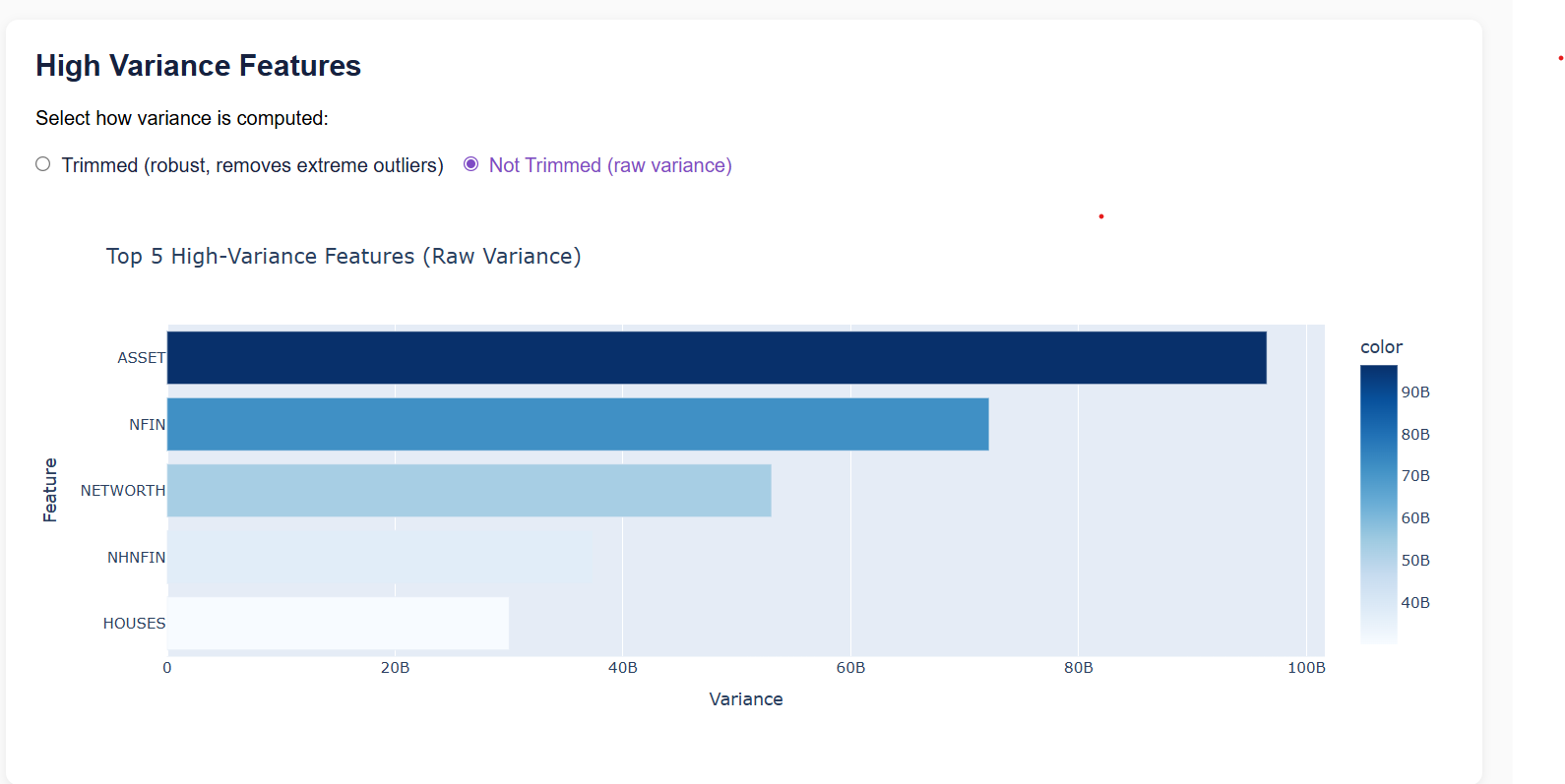
One of the dashboard's unique features is the ability to switch between raw variance and trimmed variance when selecting the most informative financial variables. This may seem like a small option, but it highlights an important concept in real-world data science.
Raw variance includes every observation, making it more sensitive to extreme outliers. Trimmed variance removes a small percentage of the highest and lowest values before calculating variance, producing a more robust estimate of variability.
Allowing users to switch between these two methods demonstrates how feature selection itself can influence the clustering process. When the variance method changes, the dashboard automatically:
- Recalculates feature rankings.
- Selects the top five financial variables.
- Retrains the K-Means model.
- Updates every visualization.
This dynamic workflow mirrors how analysts often compare multiple preprocessing strategies before settling on a final model.
Selecting the Number of Clusters
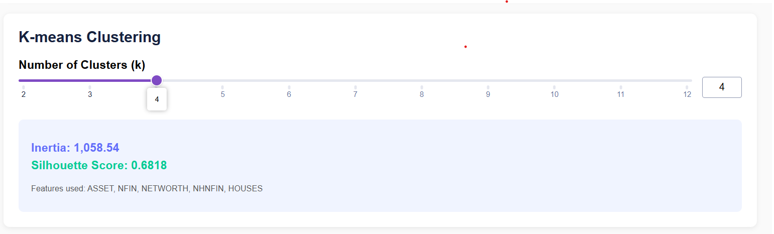
Choosing the number of clusters is one of the most important decisions in K-Means clustering. Instead of fixing this value, I added an interactive slider that allows users to select any value of K between 2 and 12.
Every time the slider changes, the application retrains the clustering model using the selected number of clusters. This provides an opportunity to observe how customer segmentation evolves as the model becomes more or less granular.
For example:
- Smaller values of K produce broader customer categories.
- Larger values create more specialized household segments.
Rather than reading about the effects of changing K, users can experience those changes instantly through the dashboard.
Live Model Evaluation
One challenge with interactive machine learning applications is helping users determine whether a clustering solution is actually good. To address this, the dashboard displays two evaluation metrics that update in real time:
- Inertia: Inertia measures how closely households are grouped around their assigned cluster centroids. Lower inertia generally indicates tighter, more compact clusters. However, inertia almost always decreases as more clusters are added, making it insufficient as the sole evaluation metric.
- Silhouette Score: The silhouette score provides a more balanced measure of cluster quality. It evaluates both: Cluster cohesion (how similar households are within the same cluster) and Cluster separation (how distinct different clusters are). Higher silhouette scores indicate that households fit well within their assigned clusters while remaining clearly separated from neighboring groups. Displaying both metrics together allows users to make more informed decisions about the appropriate number of clusters.
Visualizing Customer Segments with PCA
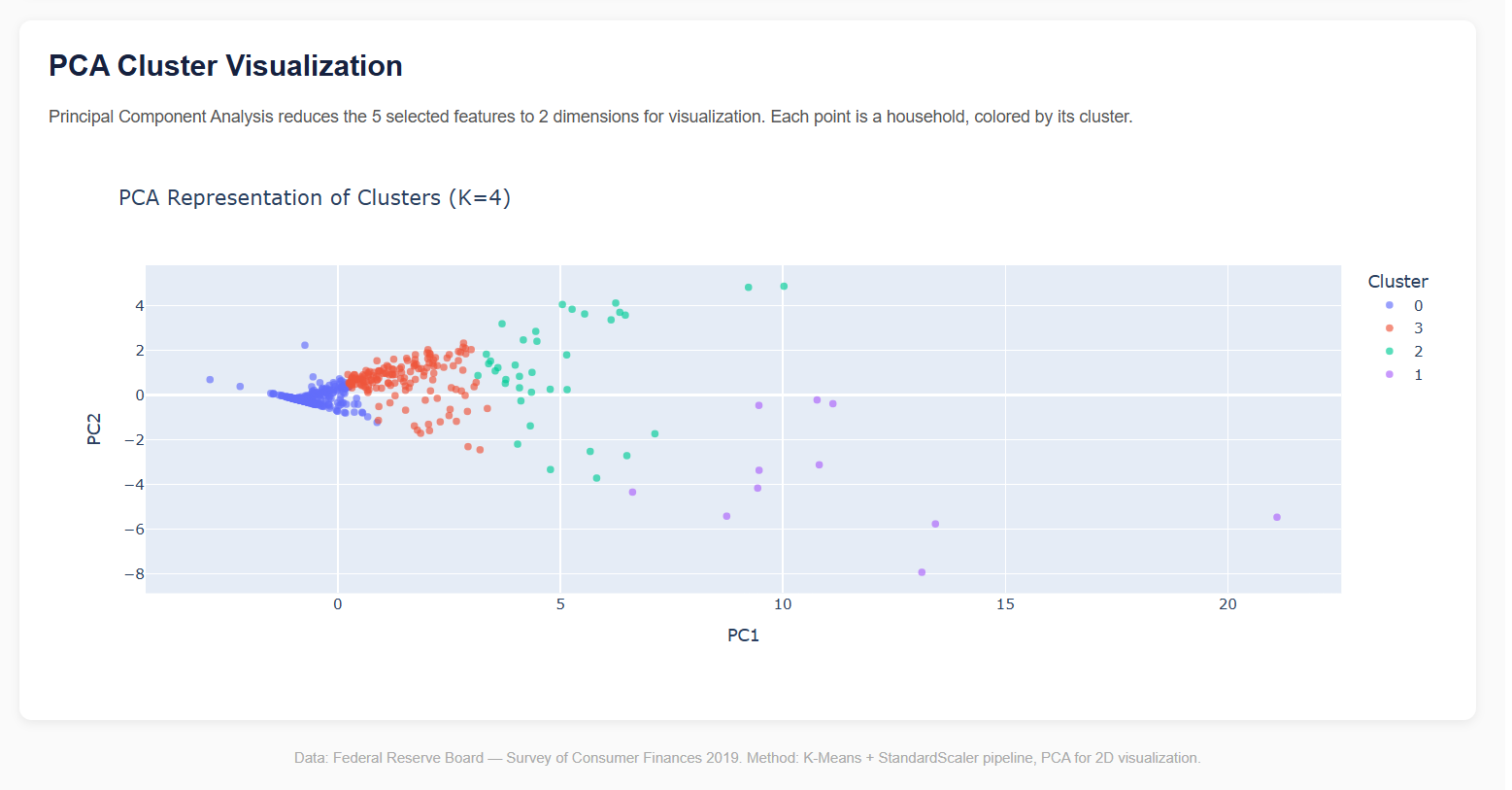
High-dimensional financial data is difficult to interpret directly. Although the clustering model uses multiple standardized financial variables, humans naturally understand two-dimensional visualizations much better.
To bridge this gap, the dashboard uses Principal Component Analysis (PCA) to project household data into two dimensions. The resulting scatter plot allows users to:
- View each household as an individual point.
- Identify distinct customer segments through color-coded clusters.
- Observe how cluster boundaries change when different values of K are selected.
- Explore household distributions interactively using hover tooltips.
This visualization transforms abstract mathematical calculations into something that is immediately understandable. Instead of looking at rows of numerical data, users can literally see the hidden structure discovered by the machine learning algorithm.
Bringing Everything Together with Dash Callbacks
One of Dash's most powerful features is its callback system. Callbacks create connections between user inputs and application outputs, allowing the dashboard to respond automatically whenever an input changes.
In this project, callbacks handle the entire machine learning workflow behind the scenes. When a user adjusts the variance method or moves the cluster slider, the application automatically:
- Selects the appropriate variance calculation.
- Identifies the top five financial features.
- Standardizes the selected variables.
- Retrains the K-Means clustering model.
- Computes updated inertia and silhouette scores.
- Applies PCA for visualization.
- Refreshes every chart and metric displayed on the dashboard.
This creates a seamless experience where users receive immediate feedback without manually rerunning notebooks or writing code. It also demonstrates how machine learning models can be integrated into interactive applications that support exploration and decision-making.
Deploying the Dashboard on Render
Once the dashboard was complete, the final step was making it accessible online. Rather than limiting the project to a local machine, I deployed the application on Render, a cloud platform that simplifies hosting Python web applications directly from GitHub repositories.
The deployment workflow was straightforward:
- The project repository was pushed to GitHub for version control.
- Render was connected to the repository.
- Dependencies were installed automatically using the requirements.txt file.
- The application launched using the Dash entry point defined in the deployment configuration.
- Future updates could be deployed automatically whenever changes were pushed to GitHub.
Hosting the dashboard online means anyone including recruiters, hiring managers, collaborators, or fellow data science enthusiasts can explore the project through a web browser without installing Python or cloning the repository.
One consideration with Render's free tier is the cold start behavior. If the application has been inactive for a period of time, the first request may take around 30-60 seconds while the service spins up. After that initial delay, the dashboard responds smoothly and behaves like a continuously running application.
Deploying the project completes the end-to-end workflow, demonstrating not only model development but also the practical skills required to package, deploy, and share machine learning solutions in a real-world environment.
Conclusion
This project goes far beyond implementing a single machine learning algorithm. It demonstrates the complete lifecycle of a modern data science solution—from exploring raw financial data and selecting meaningful features to building, evaluating, visualizing, and deploying an interactive application.
Along the way, I applied several core data science concepts, including:
- Exploratory Data Analysis (EDA) to understand household financial patterns and prepare the data.
- Feature selection using both raw and trimmed variance to identify the variables that best differentiate households while reducing the influence of outliers.
- K-Means clustering to uncover natural customer segments without relying on labeled data.
- StandardScaler to ensure all financial variables contributed equally during distance-based clustering.
- The Elbow Method and Silhouette Score to evaluate clustering quality and guide the selection of an appropriate number of clusters.
- Principal Component Analysis (PCA) to transform high-dimensional financial data into intuitive two-dimensional visualizations.
- Dash and Plotly to create an interactive web application where users can explore different clustering scenarios in real time.
- Render deployment to make the dashboard publicly accessible and demonstrate how machine learning models can be delivered as usable web applications.
Beyond the technical implementation, this project highlights an important principle of data science: generating value from data is not just about building models, it's about making insights accessible. By combining machine learning with interactive visualizations, the dashboard enables users to explore complex financial patterns, compare customer segments, and understand the impact of different modeling choices without needing to inspect the underlying code.
For me, this project was also an opportunity to strengthen skills that extend beyond machine learning itself, including feature engineering, model evaluation, data visualization, dashboard development, cloud deployment, and communicating analytical results effectively.