Back to Blog
Machine Learning August 9, 2026 25 min read
Building an End-to-End Customer Churn Prediction System with React, Django, XGBoost, and SHAP
Desire
Customer retention has become one of the biggest challenges across subscription-based industries. Whether it's telecommunications, banking, insurance, SaaS, or streaming platforms, acquiring new customers is significantly more expensive than retaining existing ones. Every customer who leaves represents not only lost recurring revenue but also the marketing and operational costs required to replace them.
This is where customer churn prediction becomes invaluable. By leveraging machine learning, organizations can identify customers who are likely to leave before they actually do, allowing customer success teams to intervene with targeted retention strategies. Rather than reacting after losing valuable customers, businesses can proactively reduce churn, improve customer satisfaction, and maximize lifetime value.
In this project, I built a full-stack Customer Churn Prediction application that combines modern web development with production-ready machine learning. The application uses a React frontend for an intuitive user interface, a Django REST Framework backend for serving predictions, and an XGBoost machine learning model trained on the IBM Telco Customer Churn dataset. To improve transparency and trust, I also integrated SHAP (SHapley Additive exPlanations), enabling users to understand why the model predicts a customer is likely to churn.
Unlike many machine learning projects that stop after model training, this project demonstrates the complete lifecycle of deploying machine learning into a real-world application — from data preprocessing and feature engineering to API development, frontend integration, explainable AI, and cloud deployment.
Before building a predictive model, it's important to understand what customer churn actually means and why businesses invest heavily in reducing it.
Customer churn refers to the percentage of customers who stop using a company's product or service during a given period. In the telecommunications industry, churn occurs when a subscriber cancels their service or switches to a competing provider.
Although losing a single customer may seem insignificant, churn can have a substantial financial impact when scaled across thousands or millions of subscribers. For example, consider a telecom provider with one million customers and an annual churn rate of just 20%. That means approximately 200,000 customers leave every year. Replacing those customers often requires expensive marketing campaigns, promotional discounts, sales commissions, and onboarding costs. Studies consistently show that acquiring a new customer can cost several times more than retaining an existing one.
This makes customer retention one of the highest-return investments a business can make. Rather than treating every customer equally, predictive analytics allows organizations to focus retention efforts on individuals who are genuinely at risk of leaving.
Instead of offering discounts to every customer — which would be both expensive and inefficient — a churn prediction model identifies high-risk customers and recommends targeted interventions such as:
This data-driven approach significantly improves marketing efficiency while increasing customer lifetime value.
Telecommunications companies generate predictable recurring revenue from monthly subscriptions. However, that business model only remains profitable if customers continue renewing their contracts.
Every customer who leaves affects multiple business metrics simultaneously:
Industry estimates suggest that replacing a churned telecom customer can cost between $1,000 and $3,000, depending on acquisition channels, promotional campaigns, and onboarding expenses. When thousands of customers churn annually, the financial impact can reach millions of dollars.
The challenge is that companies often don't know which customers are about to leave until it's too late. Traditional reporting methods focus on historical data — they tell businesses who already left. Machine learning changes this approach entirely by answering a much more valuable question: Which customers are likely to leave next? Answering this question enables organizations to move from reactive decision-making to proactive customer retention. That shift is the primary motivation behind this project.
The goal of this project wasn't simply to train an accurate machine learning model. Instead, I wanted to build an end-to-end production-ready application capable of supporting real business decisions.
The primary objectives included:
These objectives required combining several disciplines — including machine learning, backend development, frontend engineering, API design, and cloud deployment — into a single cohesive system.
One of the strengths of this project is that it demonstrates how machine learning models integrate into modern software systems rather than existing only inside Jupyter notebooks. The application follows a three-layer architecture:
The frontend serves as the user interface where users enter customer information such as:
Once submitted, the frontend sends the customer data to the backend through a REST API. The prediction results including churn probability, overall risk level, and the key factors influencing the prediction are then displayed in a user-friendly format.
React was chosen because it enables the development of responsive, component-based interfaces that are easy to maintain and scale. Combined with Vite, it also offers fast development, efficient bundling, and an excellent developer experience.
The backend acts as the bridge between the frontend and the machine learning model. Its responsibilities include:
Using Django REST Framework (DRF) allowed me to expose the machine learning model through a clean RESTful API. This separation of concerns means that the frontend and backend can evolve independently, making the system more modular and easier to maintain.
At the core of the application lies the predictive engine. This layer is responsible for:
Instead of functioning as an isolated notebook, the trained model was serialized into deployment-ready artifacts (model.pkl and preprocessor.pkl) and integrated into the backend. This approach ensures that the same preprocessing pipeline used during training is consistently applied during inference, reducing the risk of discrepancies between development and production environments.
Every successful machine learning project begins with understanding the data. Even the most sophisticated algorithms will struggle if they're trained on poorly understood or poorly prepared datasets.
For this project, I used the IBM Telco Customer Churn dataset, one of the most widely used benchmark datasets for binary classification and customer analytics. It contains information about 7,043 telecom customers and includes demographic details, account information, subscribed services, billing behavior, and whether each customer ultimately stayed with or left the company.
The objective is straightforward: predict whether a customer is likely to churn based on the characteristics available at the time of prediction.
Although the dataset is relatively small compared to enterprise-scale telecom databases, it captures many of the factors that influence customer retention, making it an excellent dataset for building and demonstrating production-ready churn prediction systems.
Each row in the dataset represents a single customer, while each column describes an aspect of that customer's relationship with the telecom company. Some variables describe who the customer is:
Other variables describe the services they subscribe to:
Several columns capture billing and account information:
Finally, the target variable indicates whether the customer stayed or churned. This mix of demographic, behavioral, and financial features makes the dataset particularly suitable for supervised machine learning because the model can learn how combinations of customer characteristics influence the likelihood of churn.
Machine learning problems generally fall into two broad categories:
Since customers either stay or leave, churn prediction is a binary classification problem. Instead of predicting a numerical quantity like monthly revenue or customer lifetime value, the model predicts one of two possible outcomes:
0 → Customer stays1 → Customer churnsAlthough the final prediction is binary, the model actually calculates a probability first.
| Customer | Churn Probability | Prediction |
|---|---|---|
| Customer A | 0.12 | Stay |
| Customer B | 0.41 | Stay |
| Customer C | 0.89 | Churn |
| Customer D | 0.97 | Churn |
These probabilities are often more valuable than the binary prediction itself. A customer with a 95% churn probability requires immediate intervention, whereas a customer with a 52% probability might simply be monitored. This is why the application returns both:
Providing richer information enables business teams to prioritize retention efforts more effectively.
EDA is the process of investigating a dataset before building machine learning models. Its purpose is to understand the structure of the data, identify potential issues, detect patterns, and generate hypotheses.
Rather than immediately training an algorithm, data scientists first ask questions such as:
Answering these questions early prevents costly mistakes later in the machine learning pipeline. For this project, the EDA stage involved visualizing customer distributions, examining churn rates across different categories, analyzing numerical relationships, and identifying variables that appeared most predictive.
By the end of the exploratory analysis, I had developed a much clearer understanding of the dataset's structure, customer behavior, and the variables most closely associated with churn. These insights laid the foundation for the next phase of the project: data cleaning and feature engineering.
One of the most underestimated stages of any machine learning project is data cleaning. While model selection often receives the most attention, the quality of a model is ultimately determined by the quality of the data it learns from. A popular saying in data science captures this perfectly: "Garbage in, garbage out."
No matter how advanced an algorithm is, it cannot produce reliable predictions if it is trained on inconsistent, incomplete, or poorly formatted data. Industry surveys consistently show that data scientists spend a significant portion of their time preparing and cleaning data rather than building models.
For this project, the data cleaning process involved addressing missing values, correcting data types, removing unnecessary information, and preparing the target variable for supervised learning.
After cleaning the data, the next stage was feature engineering. Feature engineering is the process of creating new variables from existing data to help machine learning models identify patterns more effectively.
Many beginners assume that selecting a sophisticated algorithm automatically leads to better performance. In reality, well-designed features often contribute more to model accuracy than switching from one algorithm to another. Feature engineering incorporates domain knowledge into the dataset. Instead of relying solely on raw variables, we create new features that better represent customer behavior, business risk, or operational insights.
For this project, several domain-specific features were engineered based on business understanding of customer churn. These new variables significantly enriched the dataset and improved the model's ability to distinguish between customers likely to stay and those likely to leave. The features included:
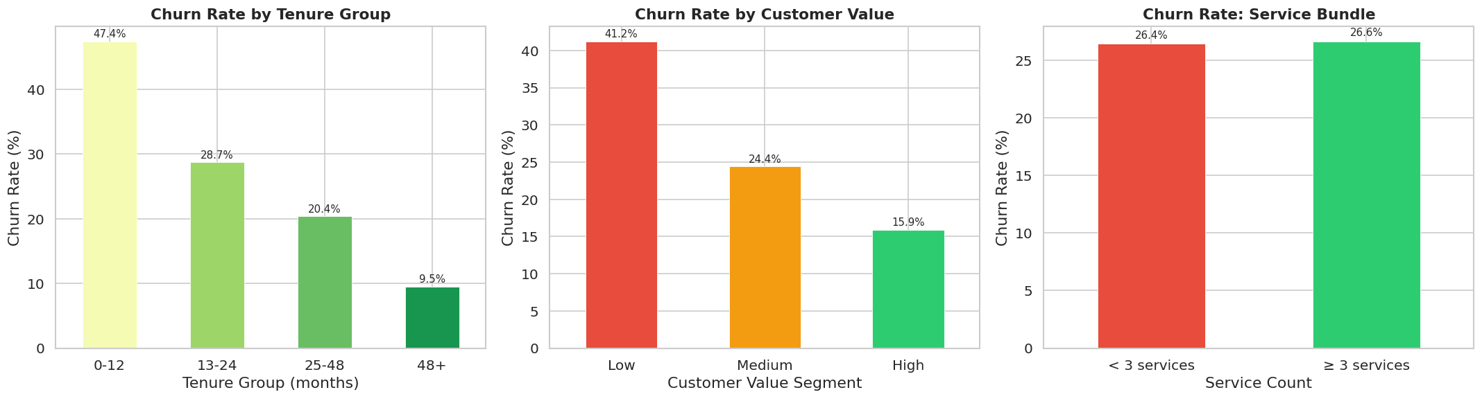
Creating new features is only worthwhile if they genuinely improve understanding of the data. After engineering these variables, I visualized each one against the target variable to verify that they captured meaningful churn patterns. The results were encouraging.
The engineered features clearly reinforced trends observed during exploratory data analysis:
These visual validations increased confidence that the engineered features were contributing meaningful information rather than introducing unnecessary complexity. Feature engineering transformed the dataset from a collection of raw customer records into a richer representation of customer behavior and business context.
One of the biggest lessons from this project is that better features frequently outperform more complicated algorithms. Many practitioners immediately search for increasingly sophisticated models, believing that higher complexity automatically leads to better performance.
However, even the most advanced algorithms can only learn from the information available. Thoughtfully engineered features expose hidden relationships, simplify complex behaviors, and incorporate domain expertise that raw data alone may not reveal. In many real-world machine learning applications, investing time in understanding the business problem and designing meaningful features produces greater performance improvements than endlessly tuning model hyperparameters.
Once the dataset had been cleaned and enriched through feature engineering, the next step was preparing it for machine learning. While this might sound straightforward, it is one of the most critical stages in any data science project.
Machine learning algorithms cannot work directly with raw data. Before a model can learn meaningful patterns, every feature must be transformed into a format that the algorithm understands. This process is known as data preprocessing.
A well-designed preprocessing pipeline ensures that data is handled consistently during both training and deployment. Without one, the model may receive inputs during production that differ from what it saw during training, resulting in unreliable predictions.
To avoid this problem, I built a preprocessing pipeline using Scikit-learn's ColumnTransformer, allowing every transformation applied during training to be saved and reused later by the Django backend. This approach ensures consistency, reproducibility, and scalability — three essential characteristics of production-ready machine learning systems.
Imagine training a model using one version of the data but sending completely different input formats during deployment. For example:
Although these differences might seem small, they can dramatically reduce prediction accuracy because the model is effectively receiving unfamiliar data. This problem is known as training-serving skew, and it is one of the most common causes of machine learning failures in production.
By saving the preprocessing pipeline alongside the trained model, every incoming customer record is transformed exactly the same way it was during training. This guarantees that the model receives data in a consistent format regardless of whether predictions are generated inside a notebook, through an API, or from a web application.
One challenge with real-world datasets is that not every feature should be processed in the same way. Consider the IBM Telco dataset. Some variables are numerical:
Others are categorical:
Some engineered features are already represented numerically and therefore require no transformation. Applying identical preprocessing to every feature would be inappropriate. This is where ColumnTransformer becomes extremely valuable.
Rather than building multiple independent preprocessing steps, ColumnTransformer allows different transformations to be applied to different subsets of columns within a single unified pipeline. Conceptually, the preprocessing workflow looked like this:
StandardScalerOneHotEncoderAlthough the workflow appears simple, it provides a significant engineering advantage. Instead of manually preprocessing every prediction request inside the backend, the entire transformation process is stored inside the serialized preprocessor.pkl artifact.
During deployment, the Django API simply loads the saved preprocessor and applies the exact same transformations before sending the data to the XGBoost model. This eliminates inconsistencies while keeping the backend code clean and maintainable.
Machine learning algorithms often perform better when numerical variables exist on similar scales. Consider these two features:
| Feature | Example Value |
|---|---|
| Tenure | 48 |
| Monthly Charges | 95 |
| Total Charges | 5,200 |
Although all three variables are important, their numerical ranges differ substantially. Some algorithms may inadvertently assign greater importance to features with larger numeric values simply because of their scale. To reduce this issue, I applied StandardScaler to selected numerical features. StandardScaler transforms each feature by subtracting its mean and dividing by its standard deviation.
The resulting values have:
This standardization allows numerical variables to contribute more evenly during model training. It's worth noting that XGBoost itself does not strictly require feature scaling because tree-based algorithms split data based on thresholds rather than distances. However, scaling was still included because:
Designing flexible preprocessing pipelines is a best practice that makes experimentation much easier in future iterations of a project.
One of the biggest challenges in customer churn prediction is that many features are categorical rather than numerical. For example:
Contract = Month-to-monthInternet Service = Fiber opticPayment Method = Electronic checkHumans understand these categories immediately. Machine learning algorithms do not. Algorithms only operate on numerical values. A naive approach might assign numbers directly:
However, this introduces an unintended mathematical relationship. The algorithm may incorrectly assume that 3 > 2 > 1 or that "No Internet" is somehow greater than "Fiber." In reality, these categories have no inherent numerical order. To solve this problem, I used One-Hot Encoding.
Instead of converting one column into numerical rankings, One-Hot Encoding creates separate binary columns for each category.
| Internet Service | Fiber | DSL | No Internet |
|---|---|---|---|
| Fiber | 1 | 0 | 0 |
| DSL | 0 | 1 | 0 |
| No Internet | 0 | 0 | 1 |
This representation preserves the categorical nature of the data while making it compatible with machine learning algorithms. Although One-Hot Encoding increases the number of features, it prevents misleading mathematical relationships and allows the model to learn independent effects for each category.
After preprocessing was defined, the dataset was divided into training and testing subsets. The split followed an 80/20 ratio:
This separation is essential because evaluating a model on the same data used for training would produce unrealistically optimistic results. Training data teaches the model and testing data evaluates whether the model has learned patterns that generalize beyond the examples it has already seen.
Rather than performing a random split, I used stratified sampling. Remember that the churn dataset is imbalanced:
A purely random split could accidentally produce:
Such discrepancies make evaluation unreliable because the testing data no longer reflects the original population. Stratified sampling preserves the class proportions in both datasets. Maintaining this balance ensures that performance metrics accurately reflect how the model is likely to behave in real-world scenarios.
With the data fully prepared, the next step was training the machine learning model. Model selection is one of the most discussed aspects of any machine learning project, but choosing the "best" algorithm isn't simply about selecting the newest or most complex option. The ideal model depends on the type of data, the business problem, and the desired balance between performance, interpretability, computational efficiency, and deployment requirements.
For this project, I selected XGBoost (Extreme Gradient Boosting), one of the most widely used algorithms for structured tabular data. XGBoost has consistently demonstrated state-of-the-art performance in data science competitions and real-world business applications, making it a strong choice for customer churn prediction.
Its popularity stems from its ability to model complex, non-linear relationships while remaining efficient enough for production environments. Since churn is influenced by multiple interacting factors such as contract type, tenure, billing behavior, and subscribed services, an algorithm capable of capturing these interactions is essential.
There are many algorithms that could be used for binary classification, including:
Each has its strengths and trade-offs. For example, Logistic Regression is highly interpretable but may struggle to capture complex, non-linear relationships. Decision Trees are intuitive but prone to overfitting. Neural Networks are powerful but often require significantly larger datasets and more computational resources.
XGBoost strikes an excellent balance between predictive performance, speed, and robustness. Some of its key advantages include:
Because the IBM Telco dataset consists primarily of structured customer records rather than images or text, XGBoost was a natural choice.
Once training was complete, the model was evaluated on the unseen test dataset. This is arguably the most important stage of model development because it measures how well the model is likely to perform in production.
Rather than relying on a single metric, I evaluated the classifier using several complementary performance measures: accuracy, precision, recall, and F1 Score. Each metric highlights a different aspect of model behavior.
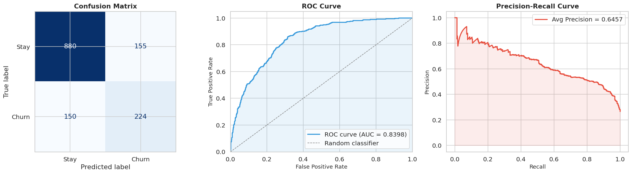
To better understand prediction outcomes, I also generated a confusion matrix. A confusion matrix summarizes predictions into four categories:
| Actual | Predicted | Outcome |
|---|---|---|
| Stay | Stay | True Negative |
| Stay | Churn | False Positive |
| Churn | Churn | True Positive |
| Churn | Stay | False Negative |
Unlike a single metric, the confusion matrix provides a complete picture of model performance. For example, it reveals:
Understanding these outcomes helps businesses evaluate the operational impact of deploying the model. For example, if retention campaigns are inexpensive, a company may accept more false positives to ensure that fewer churning customers are overlooked. Conversely, if retention offers are costly, the business may choose a higher decision threshold to improve precision.
Building an accurate machine learning model is only part of the challenge. In real-world business environments, decision-makers need confidence that a model is both reliable and understandable.
Imagine presenting a churn prediction model to a telecom company's executive team. Suppose the model predicts that a customer has an 89% probability of churning. A manager is likely to ask:
Simply responding, "The algorithm says so," isn't sufficient. Modern machine learning systems are increasingly expected to provide not only accurate predictions but also clear explanations. This is especially important in industries such as finance, healthcare, insurance, and telecommunications, where model outputs influence significant business decisions.
To evaluate the reliability of the model and make its predictions interpretable, I used two complementary approaches:
Together, these techniques help answer two critical questions:
One of the most widely used evaluation tools for classification models is the Receiver Operating Characteristic (ROC) Curve. Unlike accuracy, which measures performance at a single classification threshold, the ROC curve evaluates the model across every possible decision threshold.
Although ROC curves are extremely useful, they are not always sufficient for imbalanced datasets. Recall that approximately 73% of customers stayed and 27% churned. When one class significantly outnumbers another, Precision-Recall (PR) curves often provide a more realistic picture of performance. Instead of comparing recall and false positive rate, the Precision-Recall curve examines the relationship between precision and recall. This relationship is important because improving recall often reduces precision.
Although XGBoost delivers excellent predictive performance, it introduces another challenge. Unlike simple linear models, XGBoost consists of hundreds of interconnected decision trees. This complexity makes it difficult to explain individual predictions.
Imagine asking the model: "Why is this customer predicted to churn?" Without specialized interpretability tools, the answer would essentially be: "Because that's what hundreds of trees collectively decided."
For many organizations, this lack of transparency creates trust issues. Managers may hesitate to base retention strategies on predictions they cannot understand. This challenge is commonly known as the black box problem in machine learning.
As models become more sophisticated, their internal reasoning often becomes harder for humans to interpret. This is where Explainable AI (XAI) becomes invaluable.
Explainable AI (XAI) refers to techniques that make machine learning models easier for humans to understand. Instead of treating predictions as mysterious outputs, XAI identifies:
Explainability provides several benefits:
For churn prediction, explanations are particularly valuable because they help transform predictions into actionable retention strategies. Knowing that a customer will likely churn is useful. Knowing why they may churn is far more valuable.
To explain model predictions, I used SHAP (SHapley Additive exPlanations). SHAP is one of the most widely adopted explainability frameworks in modern machine learning.
SHAP determines how much each feature contributed to reaching that probability. Perhaps:
Rather than producing one opaque prediction, SHAP decomposes the prediction into understandable pieces. This makes complex machine learning models far more transparent.
One of SHAP's most powerful capabilities is explaining the model globally. Instead of examining one customer, global explanations summarize how the model behaves across the entire dataset.
I generated a SHAP summary (beeswarm) plot, which ranks features according to their overall importance while also showing how feature values influence predictions.
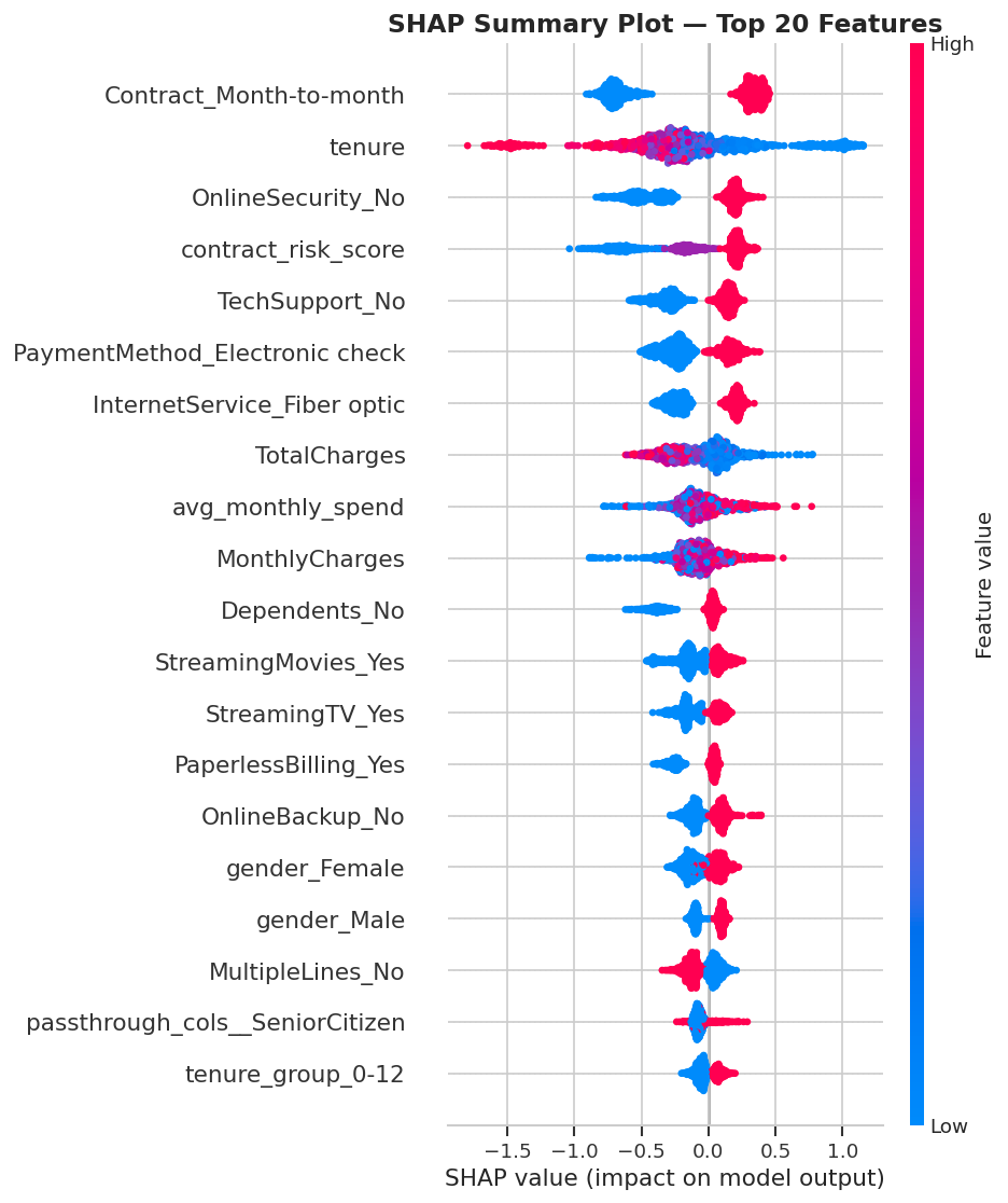
The analysis revealed several dominant churn drivers:
These findings closely matched the patterns identified during exploratory data analysis, providing strong evidence that the model was learning genuine business relationships rather than random noise.
While global explanations help us understand how the model behaves overall, businesses rarely make decisions about "average" customers. Customer retention teams work with individual customers.
When a particular customer appears at high risk of churning, decision-makers need to understand the specific reasons behind that prediction before deciding how to intervene. This is where local explainability becomes incredibly valuable. Rather than answering "What drives churn across the entire customer base?" local explanations answer "Why did the model predict that this specific customer is likely to churn?"
To provide these insights, I generated SHAP force plots and waterfall plots, both of which break down an individual prediction into the contributions made by each feature.

One of the visualizations generated during the project was the SHAP force plot. A force plot illustrates how different features influence a single prediction. The visualization begins with a baseline prediction, representing the average churn probability across all customers.
Each feature then acts like a force:
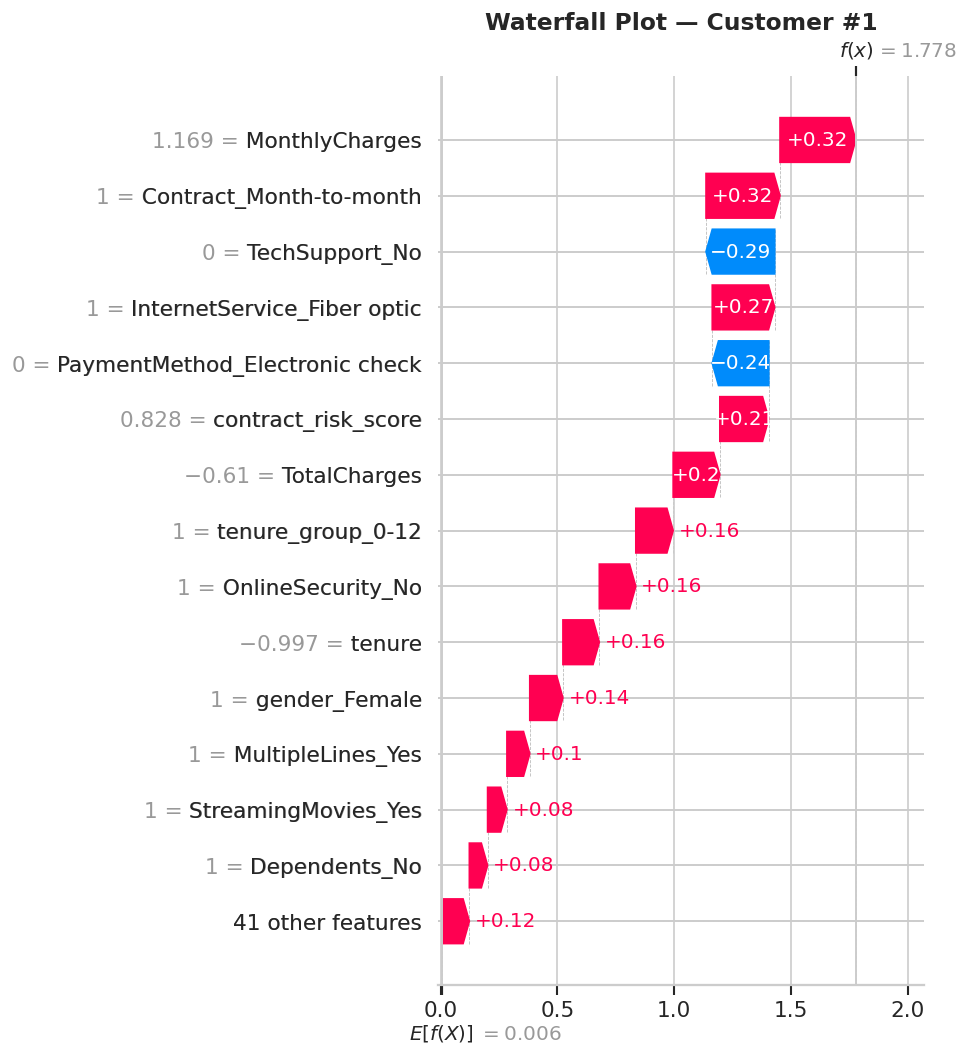
Another visualization used in the notebook was the waterfall plot. Although similar to the force plot, waterfall plots present feature contributions in a more structured sequence. The visualization starts with the baseline prediction and adds each feature one by one until the final probability is reached.
This makes it easy to answer questions like:
For analysts presenting results to business stakeholders, waterfall plots are often easier to interpret than raw numerical outputs.
Machine learning projects often focus almost entirely on predictive accuracy. However, accuracy alone is rarely enough for production systems. Imagine a customer success manager receives a list containing 5,000 customers predicted to churn. Without explanations, the list provides little practical value.
The manager still doesn't know:
Explainability transforms predictions into actionable insights.
One of the primary goals of this project was not merely to predict churn but to help businesses reduce it. Machine learning becomes most valuable when predictions lead to measurable improvements. Based on the SHAP analysis, I developed several retention recommendations:
| SHAP Finding | Business Strategy |
|---|---|
| Month-to-month contracts | Offer discounts for annual contract upgrades |
| Short tenure | Strengthen onboarding and early engagement |
| High monthly charges | Introduce loyalty pricing tiers |
| No online security | Bundle security with internet packages |
| No technical support | Improve customer support services |
| Electronic check payments | Incentivize AutoPay enrollment |
Each recommendation directly addresses one of the model's most influential churn drivers. This demonstrates how explainable AI bridges the gap between technical model outputs and strategic business decisions.
The backend serves as the central processing layer of the application. While the frontend focuses on collecting user input and displaying results, the backend is responsible for all communication with the machine learning model.
Its responsibilities include:
To implement these capabilities, I used Django REST Framework (DRF). DRF extends Django with powerful tools for building RESTful APIs, making it an excellent choice for serving machine learning models.
One challenge in deploying machine learning models is ensuring that the exact model used during training is also used in production. Retraining the model every time the server starts would be inefficient and impractical.
Instead, the trained XGBoost classifier was serialized into a file named model.pkl. Similarly, the complete preprocessing pipeline was saved as preprocessor.pkl.
During deployment, the backend loads these artifacts into memory. Whenever a prediction request arrives, the workflow becomes:
Because the preprocessing pipeline was also saved, the backend performs exactly the same transformations used during model training. This consistency eliminates training-serving skew and ensures reliable predictions.
While the backend performs the computational work, the frontend provides the user experience. I built the client application using React with Vite. React was selected because it enables developers to create reusable UI components that simplify development and improve maintainability.
Instead of refreshing entire web pages after every interaction, React updates only the components that change. This creates a smoother and faster user experience.
The application allows users to enter customer attributes such as:
Once submitted, the frontend sends the information to the backend API and displays:
Presenting results visually makes the application accessible not only to data scientists but also to business stakeholders with limited technical backgrounds.
A machine learning project only becomes truly useful when others can access it. To make the application publicly available, I deployed both the frontend and backend using Render. The repository includes a render.yaml configuration file that automates deployment.
Render creates two services:
After deployment, the workflow becomes:
This deployment pipeline demonstrates how machine learning models transition from experimentation into real-world applications that users can interact with through a browser.
Although the application performs well, several enhancements could make it even more powerful. Future improvements include:
These improvements would move the application even closer to an enterprise-grade machine learning platform.
Customer churn prediction is one of the most impactful applications of machine learning because it directly supports business growth through proactive customer retention. In this project, I built an end-to-end solution that goes far beyond model training by combining data preprocessing, feature engineering, class balancing with SMOTE, XGBoost classification, SHAP explainability, Django REST Framework, React, and cloud deployment into a single production-ready application.
The final model achieved a cross-validation ROC-AUC of approximately 0.8405 and a test ROC-AUC of approximately 0.8398, demonstrating strong predictive performance on unseen customer data. More importantly, integrating SHAP made every prediction transparent, allowing business stakeholders to understand the drivers behind churn and translate those insights into targeted retention strategies.
This project also reinforced a broader lesson: building successful AI systems requires much more than training an accurate model. It demands a deep understanding of the business problem, careful data preparation, thoughtful feature engineering, robust evaluation, explainable predictions, scalable software architecture, and reliable deployment practices.
As organizations continue investing in predictive analytics, solutions like this demonstrate how machine learning can evolve from experimental notebooks into practical applications that support real-world decision-making. By combining modern data science techniques with full-stack development, businesses can move from reacting to customer losses after they occur to proactively identifying at-risk customers, improving retention, and creating measurable long-term value.
Full-stack churn prediction platform using React, Django REST Framework, XGBoost, and SHAP. Enables telecom providers to identify at-risk customers, understand churn drivers, and support data-driven retention strategies.

Learn how to turn raw data into reliable machine learning features. Explore transformations, categorical encoding, time-series features, leakage prevention, scikit-learn pipelines, and production monitoring.
Read
Build professional Django skills with practical guidance on architecture, ORM design, APIs, security, testing, performance, deployment, and career growth.
Read
A practical guide to machine learning engineering, covering the ML lifecycle, Python workflows, model deployment, MLOps, monitoring, responsible AI, and the skills needed to build reliable production systems.
Read